The Logistic Model
It has been observed that the size of a population in year n +1 is proportional to the size of the population in year n. And this is certainly reasonable -- common sense suggests that a large population in year n will result in a large population in year n +1, and that a small population in year n will result in a small population in the following year. However, it is also commonly recognized that a given population has a ceiling -- a maximum population size beyond which the population cannot sustain itself. This ceiling is called the carrying capacity of the environment for this population. And observation has suggested that a population very close in size to the carrying capacity will turn out to have a large drop in size the following year, as the members of the population compete with one another for the scarce life sustaining resources.
The logistic model, a simple model very commonly used in population
modeling, suggests that the population size in year n +1 should
be not only proportional to the size in year n, but also proportional
to how close the population is to the carrying capacity. For simplicity
(applied mathematicians are continually looking for ways to simplify their
models, so that it becomes more practical to actually use them!) let's
express population sizes as fractions of the carrying capacity. Thus,
a population's size will be a number between 0 and 1, 1 representing the
maximum size, and 0 representing extinction. The dual proportionality
then suggests that ![]() ,
where the constant of proportionality, a, depends on various environmental
factors. Thus, the logistic model says that the function f
referred to above is
,
where the constant of proportionality, a, depends on various environmental
factors. Thus, the logistic model says that the function f
referred to above is ![]() .
Moreover, the population sizes in a sequence of years are obtained simply
by iterating this function, beginning with the population size (between
0 and 1, remember) in the starting year. In the terminology introduced
in Vignette 6: Orbits and Fixed Points, the population
sizes in any sequence of consecutive years are found by computing the orbit
of
the initial population size under the function
.
Moreover, the population sizes in a sequence of years are obtained simply
by iterating this function, beginning with the population size (between
0 and 1, remember) in the starting year. In the terminology introduced
in Vignette 6: Orbits and Fixed Points, the population
sizes in any sequence of consecutive years are found by computing the orbit
of
the initial population size under the function ![]() .
.
An Example
As an example, suppose that the constant a has the value 1.7
(based on the totality of all environmental factors, which do not enter
the model separately), and that in the year that we begin observation,
the population in question (for example the population of red-eyed vireos
in the Chagrin Valley) is exactly 72 percent of the carrying capacity.
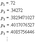
We begin iteration of the function ![]() with
the value x = .72, and find that the population sizes in subsequent
years are
with
the value x = .72, and find that the population sizes in subsequent
years are

In case you have forgotten how to do this with your TI-83 calculator, here's a quick review:

A Stable Orbit
What is of special interest in this particular example is that, although
the population declined dramatically in going from the first year to the
second year, the population begins to stabilize in subsequent years.
In fact, after the 17th year, the population has stabilized
at .4117647059. (In the terminology introduced in Vignette
6, the number .4117647059 is an attracting fixed point for the
function ![]() .
)
.
)
Is this behavior unusual? Try it with the function f (x) = 2.1x(1 - x) and an initial population size of .15. You should get a stable population of .5238095238 after about 13 steps. Try it with a = 2.1 or a = 1.7, and various other starting population sizes. The result should be a stable population after some number of iterations, in all such cases. In fact, for a given value of a, it doesn't matter what the initial population size is -- for all initial sizes (strictly between 0 and 1, of course), the population will eventually stabilize at the same size!! (This is because there is an attracting fixed point.) The biological interpretation is that, for this model, only the environmental factors are important in determining the long-range population size -- the original population size is irrelevant!
Periodic Orbits
Now try the logistic population model f (x) = 3.2x(1 - x) , with an initial population size of .15. You should find that, after sufficient iteration, the population size alternates between two values: .7994554905 and .5130445095. In fact, the initial population size is once again irrelevant. Try it with any initial population size (but keep a = 3.2), and you should get the same alternating population sizes. These population sizes form what is called an attracting cycle of period 2. This "period 2" behavior occurs with all values of a between (approximately) a = 3 and a = 3.4.
What about other values of a? Try a = 3.5, and any initial population size. That is, iterate the function f (x) = 3.5x(1 - x), starting with any initial x value. You should find the orbit being attracted to a cycle of period 4, specifically, .8269407066, .5008842103, .8749972636, and .382819683. Biologically speaking, a population for which this is an appropriate model will settle into a pattern in which the population size cycles through these four rather widely different sizes in each 4-year period.
Chaos
Not all values of a lead to stable or even periodic behavior.
For instance, try the same experiment with a = 3.7. This value
of a -- not all that much different from the a = 3.5 that
gave us a cycle of period 4 -- leads to strikingly different long-range
behavior of the population. For a population with a = 3.5,
there is absolutely no regularity to the population sizes in subsequent
years. Virtually all possible population sizes between approximately
.25 and .92 will be taken on by this population, if we wait long enough.
Moreover, the size of the population in any given year now seems to be
very highly dependent on the initial population size, a situation totally
unlike the regular, periodic behavior that we noticed for the other values
of a that we have considered. As an example, consider one
population with a = 3.7 and initial population size .41, and a second
population with a = 3.7, but initial size .42. The population
sizes in subsequent years are as follows, as you can verify easily using
your own calculator:
| Year | Population 1 | Population 2 |
| 1 | .41 | .42 |
| 2 | .89503 | .90132 |
| 3 | .3476198067 | .3290863531 |
| 4 | .8390870237 | .8169175436 |
| 5 | .4995739643 | .553384101 |
| 6 | .9249993284 | .9144555097 |
| 7 | .2566896121 | .2894385327 |
| 8 | .705960204 | .7609563134 |
| 9 | .7680474591 | .6730366693 |
| 10 | .6591570707 | .814215751 |
| 11 | .8312753993 | .5596933088 |
| 12 | .5189494562 | .9118158229 |
| 13 | .923671397 | .2975085937 |
| 14 | .2608594252 | .7732897523 |
As you can see, although the populations start off fairly close in size, after about ten years they are quite different. And by 12 or 13 years, they are so different that there is no relationship whatsoever. Rather than having stable or periodic behavior, as we observed in the logistic model with values of a equal to 1.7, 2.1, 3.2 and 3.5, the behavior we observe with a = 3.7 is what is called chaotic. One of the biological ramifications of chaos is that if we cannot measure the initial population size with total accuracy, then there is absolutely no hope of long-range prediction of the future of the population! In the above example, our two populations differed by only a small amount -- an amount that could easily be due to an error in measurement -- and then progressed in highly different ways.
The Pattern of Periodicity and Chaos
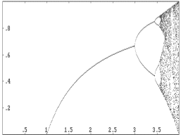
The relationship between the value of a in the logistic model f (x) = ax(1 - x) and the periodicity or chaos within the model can be visualized by a computer-generated picture. In the image below, the horizontal axis depicts the possible values of a, and the vertical axis shows the values taken on by f at long range -- after the first 50 years. For values of a for which there is only one point directly above, the population will stabilize at the size shown by the vertical axis. If there are two points above an a-value, then the population size is attracted to a cycle of period 2, and so on. The values of a for which there is a total jumble of points above are those for which the logistic model is chaotic. This type of picture is sometimes referred to as a Feigenbaum plot, in honor of Mitchell Feigenbaum, who discovered the universality of chaos in the mid 1970's, using a calculator!

In this picture, we have limited the values of a to ![]() ,
because values outside this range will cause the logistic model to yield
population sizes below 0 or above 1, both of which are impossibilities
in our understanding of the model.
,
because values outside this range will cause the logistic model to yield
population sizes below 0 or above 1, both of which are impossibilities
in our understanding of the model.
Chaos is Everywhere
Mathematicians were at first shocked by the discovery of chaotic behavior in models that are as simple as the logistic model. The logistic model is simply a quadratic function; and if functions as simple as quadratics can exhibit chaotic behavior, then more complex systems must certainly have chaotic properties as well. Today the presence of chaos is an accepted fact of mathematics and science, and one of the challenges for those fields is the discovery of how to actually use our understanding of chaos to help us to understand complex systems. The study of chaotic behavior in iterated systems is today still in its infancy, and a complete understanding of it may still be decades away.
Further Exploration